
[논문] 3D human pose estimation in video with temporal convolutions and semi-supervised training
이 논문은 FAIR팀이 CVPR 2019에 제출한 논문으로, SOTA를 달성하였다. ICCV 2019의 Exploting Spatial-temporal Relationships for 3D Pose Estimation via Graph Convolutional Networks 의 이전 SOTA이다.
그럼에도, 논문을 읽다보면 알겠지만 ICCV의 것은 $T=3$일 때이고, 따라서 본 논문의 구조 역시 $T=3$일 때를 기준으로 평가했는데, 본 논문은 $T=243$일 때를 메이저하게 다루고 있어 이 둘을 비교하는 것이 적절한지는 모르겠다.
일단 한 번 살펴보자.
이 논문을 읽기 위해 최소한 준비해야 할 것(뇌피셜)
- 알아야 할 개념: TCN
주의! 본 포스팅은 논문을 번역하거나 자세하게 설명하는 것이 아닌, 주요한 부분들을 집어 제 나름대로의 이해를 바탕으로 서술한 것입니다. 이 포스팅은 논문 이해에 도움이 될 순 있어도 논문의 모든 것을 담지 않았으니, 반드시 원문을 함께 읽으시길 바랍니다.
https://arxiv.org/pdf/1811.11742.pdf
Introduction
Introduction을 요악하면 다음과 같다.
- dilated convolution을 이용한 temporal convolution 모델로 SOTA를 달성했다.
- 근데 이게 CNN이다보니 RNN보다 훨씬 빠르고 가볍다.
- 3D Pose Estimation분야에 있어서 쓸 만한 semi-supervised 학습 방법을 발견했다.ii. 필요에 따라 외부 파라미터를 쓸 수도 있다.
- 3D annotation 없이 2D annotation과 카메라 내부 파라미터만 알면 된다.
Related Work
Related Work는 크게 Two-step pose esimation, Video pose estimation, Semi-supervised training, 3D shape recovery를 다루고 있다. Related Works의 챕터들은 해당 논문에서 이야기하는 것과 상당히 관련돼 있으니, 큰 틀에 있어서 분야적인 감을 잠을 수 있다.
Two-step pose estimation
딥러닝을 통한 3D Pose Estimation에는 크게 3가지 접근법이 있는데,
- 이미지 → 3D Pose 의 end-to-end 방식
- 이미지 + 2D Pose → 3D Pose의 Lifting 방식
- 2D Pose → 3D Pose의 Lifting 방식
등이 있다.
1번은 상당히 직관적이다. 당연히 feature extraction을 위한 ResNet등이 동반된다. 주로 Heatmap을 통한 방법이 많으며, 관련된 연구로는 3D Human Pose Estimation with 2D Margianl Heatmaps이나, MeTRAbs: Metric-Scale Truncation-Robust Heatmaps for Absolute 3D Human Pose Estimation 등이 있다.
2번은 1번에서 먼저 2d pose를 예측하고, 이미지 feature와 2d pose를 함께 사용하여 최종적으로 3d pose를 예측하는 방법이다.
3번은 오로지 2d pose 예측 혹은 ground-truth값을 입력으로 삼아 3d pose를 예측하는 방법이다.
이 두 영역에 해당하는 논문은 본 논문을 포함하여 Exploting Spatial-temporal Relationships for 3D Pose Estimation via Graph Convolutional Networks, Deep Kinematics Analysis for Monocular 3D Human Pose Estimation 등이 있다.
일반적으로 2번, 3번이 여기서 말하는 two-step pose estimation으로 함께 묶인다.
3번에서 모델 성능 평가는 Ground-Truth 입력으로 하지 않고, estimated 2d pose를 입력으로 삼는다. 보통 2, 3번에서 2d pose 예측 모델로 Stacked Hourglass모델이 상당수 채택되어 왔는데, 요즘에는 본 논문에서 밝혔듯 Cascaded Pyramid Network나 Mask R-CNN 모델이 더 효과적이기에 그것들을 사용한다.
Video pose estimation
3D Pose Estimation에는 또 다른 종류의 2가지 접근법이 있는데,
- 이미지 → 3D Pose
- 비디오 → 3D Pose
이다.
1번은 직관적으로 알 수 있듯, 이미지 한 장으로부터 하나의 3d 좌표값들을 예측하는 것이다.
2번은 예측하고자 하는 어떤 프레임의 전후 n개씩(혹은 real-time의 경우 전 2n개) 정보를 가져와 같이 활용하는 것이다. 이 논문은 이미지 없이 오직 2d pose만을 이용해 3d pose를 구하는 것인데, 한 프레임의 2d pose만 있으면 그것으로부터 제대로 된 3d pose를 구하는 것은 (앞뒤 좌우가 구분이 안가므로) 상당히 어렵다. 따라서 본 논문은 2d pose의 변화를 통해 3d pose를 구하는 논문이므로, video pose estimation의 범주에 속한다.
나머지는 별 것 없으므로 넘어가겠다.
Temporal dilated convolutional
이 논문의 자랑 중 하나는 fully convolutional architecture라는 것인데, 그것이 바로 여기서 이야기하는 temporal convolutional 덕분이다. 사실 dilated convolution + 1d convoltion + time series data로 이러한 구성을 짜는 것은 본 논문이 처음이 아니다.
처음이 어디서인지는 모르겠으나, WaveNet이 이걸로 유명하다.(이게 처음일 수도 있다.) dilated convolution으로 receptive field를 늘려 RNN없이도 효율적으로 높은 성능을 얻어낼 수 있다. 요즘은 이걸 TCN(Temporal Convolutional Network)이라고도 한다.

Figure 1은 T=9의 예시이다. T=3^k일 때 dilated convolution층이 k개만큼 존재한다.
데이터가 흐르는 모습은 딱 1d convolution인 것으로 감이 올 것이다. 이 방식은 T개의 프레임에 대한 데이터를 모두 버리지 않으면서도, 파라미터의 개수 감소와 연산 속도의 증가를 크게 이루었다.(dilated conv의 장점이다.)
디테일하게 설명하자면, 샘플 하나(이미지 1프레임에 대한 2d/3d pose값)의 tensor shape은 $(J, 2), (J, 3)$이다. $J$는 예측하고자 하는 관절의 개수인데, 일반적으로 14/15/17/19/21/28/31...등의 개수를 예측한다.
연속된 $T$개의 프레임이 있다고 할 때 다시 shape은 $(T, J, 2), (1, J, 3)$이 된다. $T$개의 2d데이터로부터 하나의 3d데이터를 예측하는 것이다.
이러한 clip? chunk?단위를 하나의 샘플로로 했을 때, x/y shape은 결국 배치사이즈 $N$에 대하여 $(N, T, J, 2)$ → $(N, 1, J, 3)$이 되는 것이다.
당연하게도 이는 CNN이기 때문에, $(T+k,J,2)$ shape의 입력이 있으면 출력은 $(1+k, J, 2)$가 된다. 그러나 본 논문의 부록에서 말하듯, Batch Norm을 위해서 그다지 선호하는 방법은 아니다.
Convolution의 진행은, 1d conv에 대해서 $T$에 관한 축(시간축)을 입력 길이로, $J$에 관한 축(관절 축)을 채널 개수로 삼는다. 이때 $(T, J, 2)$의 입력을 $(T, J\times2)$으로 바꾼다.
예를 들어 $T=9, J=15$인 경우 길이 9, 채널 개수 30인 데이터를 하나의 샘플로 입력받는 것이다.
그 다음은 dilated convs를 통과하며 길이가 9 → 3 → 1이 되어 예측을 하는 것이다.
$T=243$인 경우에는 243 → 81 → 27 → 9 → 3 → 1이 될 것이다.
본 논문에서는 입력층의 채널을 $J\times2$, 출력층의 채널을 $J\times3$으로 지정하여 최종적으로 reshape을 통한 $(N, 1, J, 3)$의 출력을 얻는다. 그 사이의 conv 채널 $C$나 receptive field $T$는 정하기 나름인데, 논문에서는 $C=1024, T=243$으로 설정하였다.


CNN의 input length → output length 공식은 아래와 같다.

커널 길이는 3으로 고정이고, stride=1, padding=0인 상황에서, dilation rate가 1 → 3 → 9 → 27 → 81로 점점 증가하므로 레이어를 거치는 tensor의 길이 역시 241 → 235 → 217 → 163 → 1로 줄어든다.
여기에 slicing을 통한 skip connection을 더해주고, 적절한 BN과 1x1 conv, dropout, relu등을 곁들이면 이 논문에서 제시하는 모델이 완성된다.
Semi-supervised approach
모델 구조는 위까지가 전부고, 지금부터는 모델 학습 방법론이다.
먼저 3d gt label이 있는 비디오의 경우, pose model에서 root-relative 좌표를 예측한다. (root 관절 - 일반적으로 pelvis - 의 좌표는 0이 된다.) 그리고 root 좌표는 trajectory model로 따로 예측한다. 나중에 이 둘을 합치면 실제 좌표를 구하는 것이다.

그리고 semi-supervised 방법론에서는, pose model과 trajectory model에서 도출한 3차원 좌표값을, 카메라 내/외부 파라미터를 통해 다시 2차원으로 투영하여 입력된 2d label과의 차이를 구한다. 3d 데이터가 적절히 예측되었다면, 2d 좌표로 다시 투영했을 때 2d label과 차이가 없어야 한다.
본 논문은 MPJPE(mean per joint position error)나 그를 기반으로 하는 WMPJPE(Weighted MPJPE)를 loss로 사용했다.
Experimental setup이나 기타 결과는 생략한다.(적당히 SOTA를 달성했다.) 디테일은 논문을 직접 읽어보길 바란다.
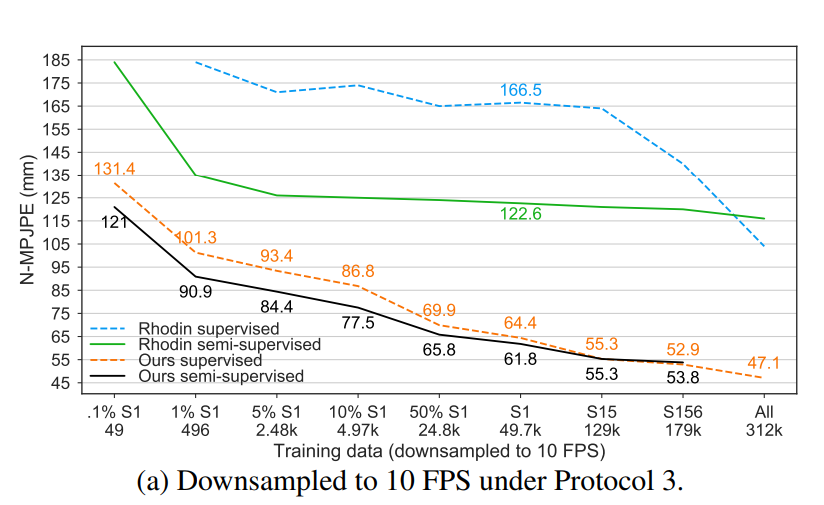
- semi-supervised approach의 효과

|

- Temporal Convolution의 효과

Parameters는 모델 파라미터의 개수, FLOPs는 부동소수점연산의 횟수를 말한다.
더 자세한 내용과 구현 코드는 저자의 페이지에서 찾아볼 수 있다.
코드를 보면 알겠지만, SOTA를 달성한 주제에 모델 구조가 꽤 간단하다...
아래 코드는 FAIR팀에게 저작권이 있다.
import torch.nn as nn

from common.memory import check_memory

class TemporalModelBase(nn.Module):
    def __init__(self, num_joints_in, in_features, num_joints_out, out_features,
                 filter_widths, causal, dropout, channels):
        super().__init__()

        for fw in filter_widths:
            assert fw % 2 != 0, 'Only odd filter widths are supported'

        self.num_joints_in = num_joints_in
        self.in_features = in_features
        self.num_joints_out = num_joints_out
        self.out_features = out_features
        self.filter_widths = filter_widths

        self.drop = nn.Dropout(dropout)
        self.relu = nn.ReLU(inplace=True)

        self.pad = [ filter_widths[0] // 2 ]
        self.expand_bn = nn.BatchNorm1d(channels, momentum=0.1)
        self.shrink = nn.Conv1d(channels, num_joints_out * out_features, 1)


    def set_bn_momentum(self, momentum):
        self.expand_bn.momentum = momentum
        for bn in self.layers_bn:
            bn.momentum = momentum

    def receptive_field(self):
        frames = 0
        for f in self.pad:
            frames += f
        return 1 + 2*frames

    def total_causal_shift(self):
        frames = self.causal_shift[0]
        next_dilation = self.filter_widths[0]
        for i in range(1, len(self.filter_widths)):
            frames += self.causal_shift[i] * next_dilation
            next_dilation *= self.filter_widths[i]
        return frames

    def forward(self, x):
        assert len(x.shape) == 4, f'input: {x.shape}'
        assert x.shape[-2] == self.num_joints_in, f'{x.shape}, {self.num_joints_in}'
        assert x.shape[-1] == self.in_features
        sz = x.shape[:3]
        x = x.view(x.shape[0], x.shape[1], -1)
        x = x.permute(0, 2, 1)
        x = self._forward_blocks(x)

        x = x.permute(0, 2, 1)
        x = x.view(sz[0], -1, self.num_joints_out, self.out_features)
        del sz
        return x

class TemporalModel(TemporalModelBase):
    def __init__(self, num_joints_in, in_features, num_joints_out, out_features,
                 filter_widths, causal=False, dropout=0.25, channels=1024, dense=False):
        super().__init__(num_joints_in, in_features, num_joints_out, out_features, filter_widths, causal, dropout, channels)

        self.expand_conv = nn.Conv1d(num_joints_in*in_features, channels, filter_widths[0], bias=False)

        layers_conv = []
        layers_bn = []

        self.causal_shift = [ (filter_widths[0]) // 2 if causal else 0 ]
        next_dilation = filter_widths[0]
        for i in range(1, len(filter_widths)):
            self.pad.append((filter_widths[i] - 1)*next_dilation // 2)
            self.causal_shift.append((filter_widths[i]//2 * next_dilation) if causal else 0)

            layers_conv.append(nn.Conv1d(channels, channels,
                                         filter_widths[i] if not dense else (2*self.pad[-1] + 1),
                                         dilation=next_dilation if not dense else 1,
                                         bias=False))
            layers_bn.append(nn.BatchNorm1d(channels, momentum=0.1))
            layers_conv.append(nn.Conv1d(channels, channels, 1, dilation=1, bias=False))
            layers_bn.append(nn.BatchNorm1d(channels, momentum=0.1))
            next_dilation *= filter_widths[i]

        self.layers_conv = nn.ModuleList(layers_conv)
        self.layers_bn = nn.ModuleList(layers_bn)

    def _forward_blocks(self, x):
        x = self.drop(self.relu(self.expand_bn(self.expand_conv(x))))
        for i in range(len(self.pad) - 1):
            pad = self.pad[i+1]
            shift = self.causal_shift[i+1]
            res = x[:, :, pad + shift : x.shape[2] - pad + shift]

            x = self.drop(self.relu(self.layers_bn[2*i](self.layers_conv[2*i](x))))
            x = res + self.drop(self.relu(self.layers_bn[2*i + 1](self.layers_conv[2*i + 1](x))))
            del pad, shift, res

        x = self.shrink(x)
        return x

class TemporalModelOptimized1f(TemporalModelBase):
    def __init__(self, num_joints_in, in_features, num_joints_out, out_features,
                 filter_widths, causal=False, dropout=0.25, channels=1024):
        super().__init__(num_joints_in, in_features, num_joints_out, out_features, filter_widths, causal, dropout, channels)
        self.rf = 1
        for f in filter_widths:
            self.rf *= f
        self.expand_conv = nn.Conv1d(num_joints_in*in_features, channels, filter_widths[0], stride=filter_widths[0], bias=False)

        layers_conv = []
        layers_bn = []

        self.causal_shift = [ (filter_widths[0] // 2) if causal else 0 ]
        next_dilation = filter_widths[0]
        for i in range(1, len(filter_widths)):
            self.pad.append((filter_widths[i] - 1)*next_dilation // 2)
            self.causal_shift.append((filter_widths[i]//2) if causal else 0)

            layers_conv.append(nn.Conv1d(channels, channels, filter_widths[i], stride=filter_widths[i], bias=False))
            layers_bn.append(nn.BatchNorm1d(channels, momentum=0.1))
            layers_conv.append(nn.Conv1d(channels, channels, 1, dilation=1, bias=False))
            layers_bn.append(nn.BatchNorm1d(channels, momentum=0.1))
            next_dilation *= filter_widths[i]

        self.layers_conv = nn.ModuleList(layers_conv)
        self.layers_bn = nn.ModuleList(layers_bn)

    def _forward_blocks(self, x):
        x = self.drop(self.relu(self.expand_bn(self.expand_conv(x))))

        for i in range(len(self.pad) - 1):
            res = x[:, :, self.causal_shift[i+1] + self.filter_widths[i+1]//2 :: self.filter_widths[i+1]]

            x = self.drop(self.relu(self.layers_bn[2*i](self.layers_conv[2*i](x))))
            x = res + self.drop(self.relu(self.layers_bn[2*i + 1](self.layers_conv[2*i + 1](x))))

        x = self.shrink(x)
        return x